6 Multivariate analyses

First load the required packages and data. Note that from the univariate analyses the analysis data set for the lab parameters has been updated to include transformed variables. Therefore, we load the second iteration of the data data/ADLB_02.rds.

6.1 V1: Association with structural variables

Attached the required structural variables to the lab data.

A scatterplot of each predictor with age, with different panels for males and females have been constructed. Associated Spearman correlation coefficients have been computed.

The remaining predictors are reported in appendix Section F.1.

6.1.1 Key predictors

6.1.2 Predictors of medium importance

6.2 V2: Correlation coefficients between all predictors

Calculate correlation matrix using Spearman correlation coefficient.

The Spearman correlation coefficients are depicted in a quadratic heat map:

6.2.1 VE1: Comparing nonparametric and parametric predictor correlation

Plot the matrix of differences between Spearman and Pearson pairwise correlation coefficients.

Plot the matrix of differences between Spearman and Pearson pairwise correlation coefficients but suppress differences less then 0.1 in absolute value.

Predictor pairs for which Spearman and Pearson correlation coefficients differ by more than 0.1 correlation units in absolute value will be depicted in scatterplots. First report the table of predictor pairs where the difference (column r) is greater than 0.1.

x	y	r
PLT	LYMR	0.12
MONO	MONOR	0.18
BASO	EOS_T	0.12
BUN	AGE	0.13
EOSR	LYMR	0.18
EOSR	EOS_T	0.21
EOSR	LYM_T	0.14
LYMR	MONOR	0.11
LYMR	EOS_T	0.17
LYMR	LYM_T	0.22
MONOR	LYM_T	0.13
NEU	NEUR	0.11

Then plot the scatter plots.

6.2.2 VE2: Variable clustering

A variable clustering analysis has been performed to evaluate which predictors are closely associated. The dendrogram groups predictors by their correlation.

This can also be displayed as a network plot:

In the following scatterplots we show predictor pairs with Spearman correlation coefficients greater than 0.8:

6.2.3 VE3: Redundancy

Variance inflation factors (VIF) will be computed between the candidate predictors. This will be done for the three possible candidate models, and using all complete cases in the respective candidate predictor sets. Since $VIF = (1-R^2)^{-1}$, we also report the multiple R-squared values.

Redundancy was further explored by computing parametric additive models for each predictor in the key predictor model and the extended predictor model. VIFs and multiple $R^2$ are reported from those models, again for the three predictor sets.

Note, the all predictor model is reported in appendix Section F.2.

6.2.3.1 VIF for key predictor model

The available sample size is 13793 (1.44 %).

Parameter code	Variance inflation factor	Multiple R-squared
SEX	1.1	0.05
PLT	1.2	0.15
BUN	2.4	0.58
NEU	5.4	0.82
AGE	1.1	0.09
CREA_T	2.3	0.56
WBC_T	5.6	0.82

6.2.3.2 VIF for model with key predictors and predictors of medium importance

The available sample size is 9389 (0.98 %).

Parameter code	Variance inflation factor	Multiple R-squared
SEX	1.1	0.09
PLT	1.4	0.30
FIB	2.3	0.56
POTASS	1.1	0.10
BUN	2.6	0.61
CRP	2.2	0.54
NEU	5.9	0.83
AGE	1.2	0.15
ALAT_T	3.3	0.69
ASAT_T	3.2	0.69
CREA_T	2.4	0.58
GGT_T	1.4	0.30
WBC_T	6.0	0.83

6.2.3.3 VIF for all predictor model

See appendix Section F.2.

6.2.3.4 Redundancy by parametric additive model: key predictor model

The available sample size is 13793 (1.44 %).

Parameter code	Variance inflation factor	Multiple R-squared
SEX	1.1	0.11
PLT	1.2	0.16
BUN	2.6	0.61
NEU	11.5	0.91
AGE	1.3	0.21
CREA_T	2.4	0.58
WBC_T	13.7	0.93

6.2.3.5 Redundancy by parametric additive model: key predictors and predictors of medium importance

The available sample size is 9389 (0.98 %).

Parameter code	Variance inflation factor	Multiple R-squared
SEX	1.2	0.15
PLT	1.5	0.32
FIB	2.4	0.58
POTASS	1.1	0.11
BUN	2.8	0.65
CRP	2.3	0.56
NEU	14.1	0.93
AGE	1.4	0.29
ALAT_T	3.4	0.70
ASAT_T	3.5	0.71
CREA_T	2.5	0.60
GGT_T	1.5	0.35
WBC_T	16.4	0.94

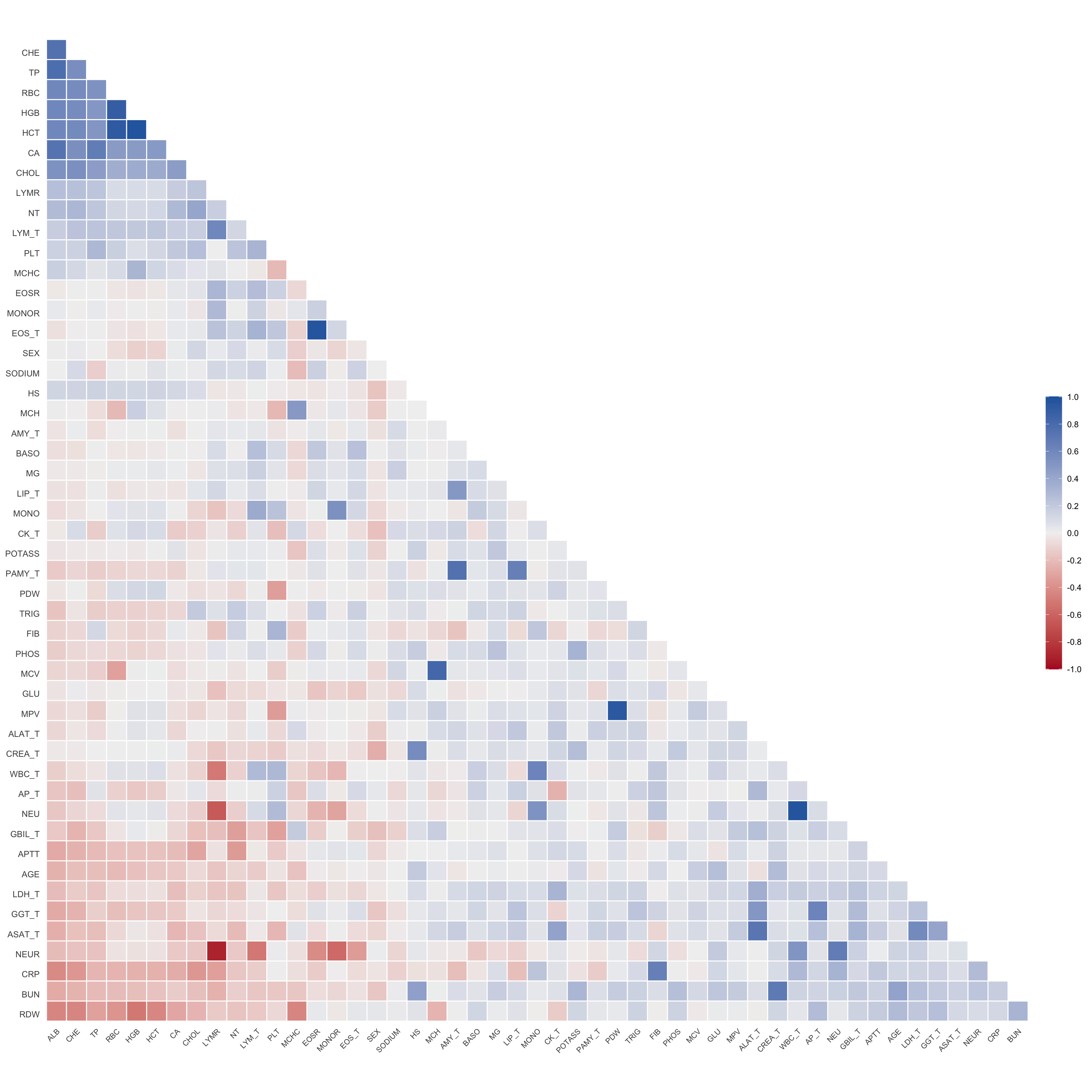
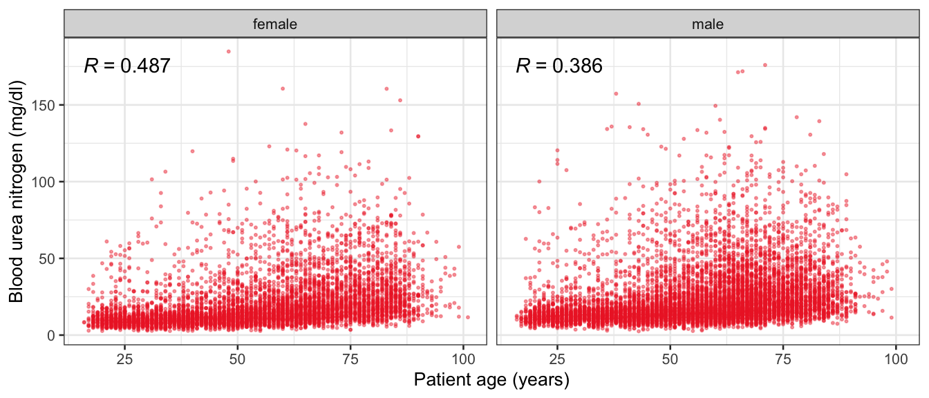
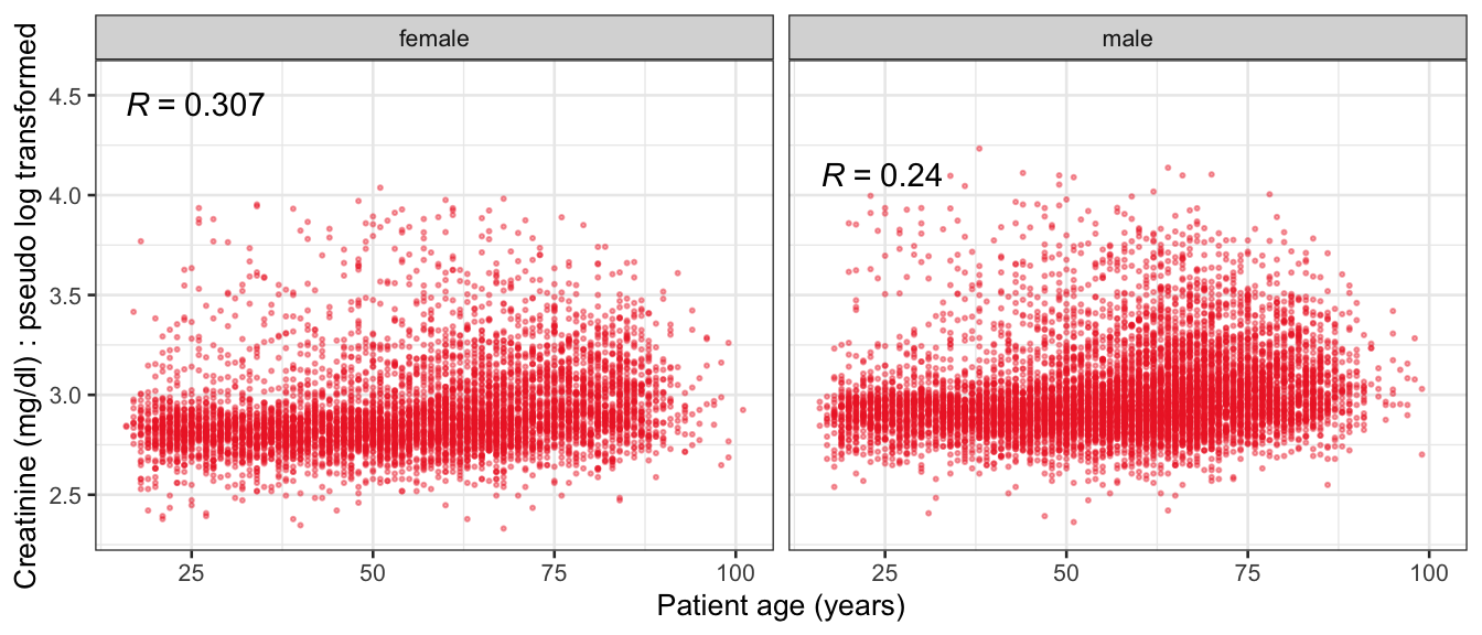
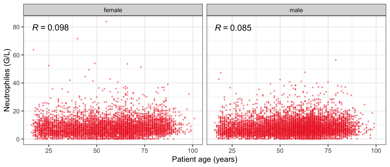
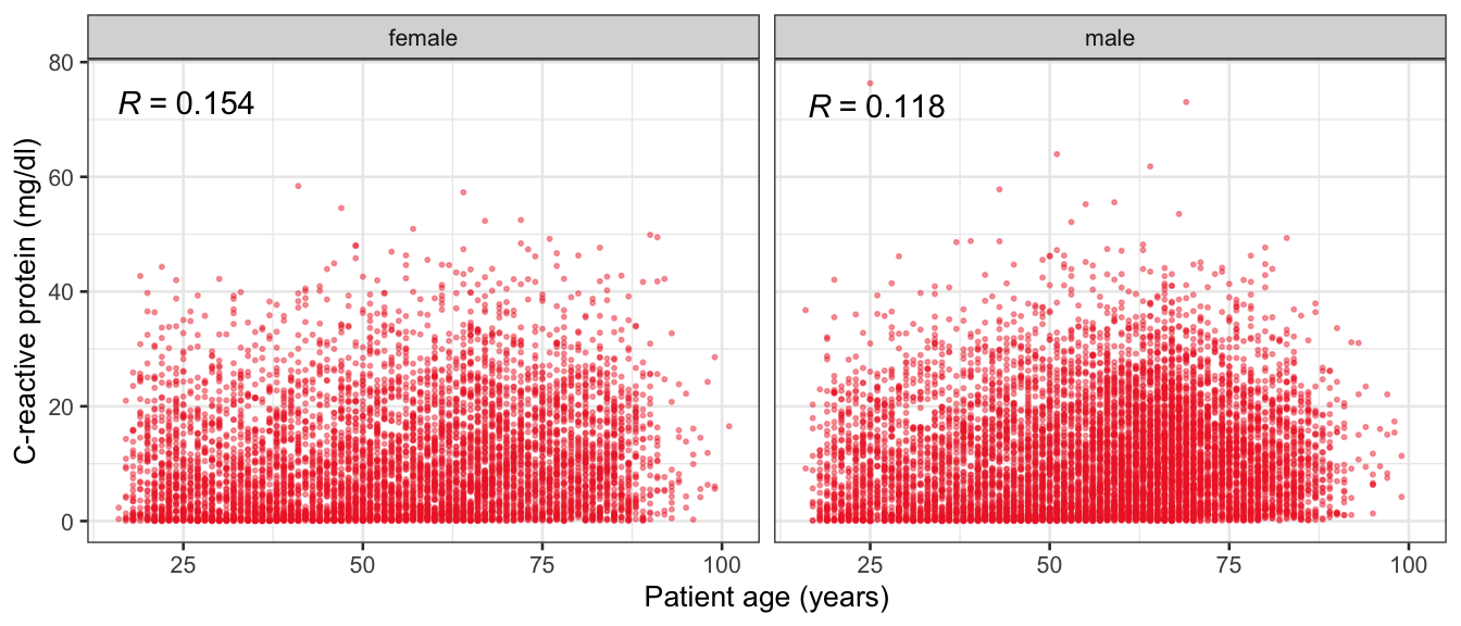
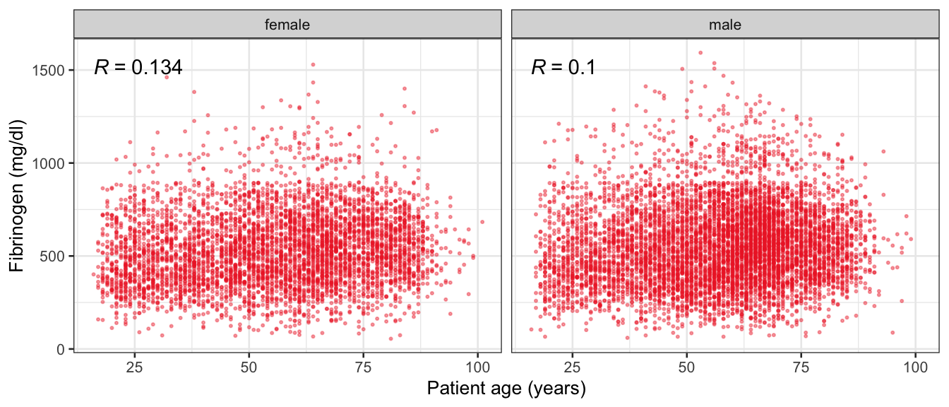
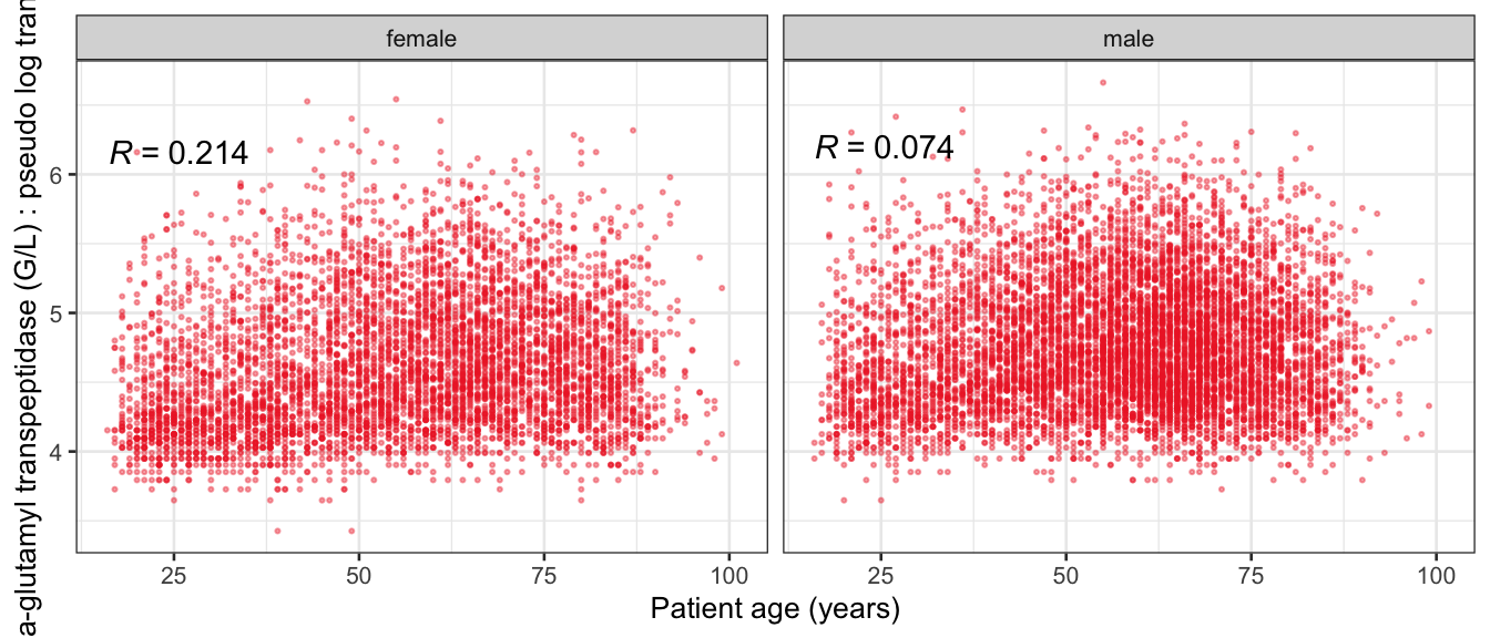
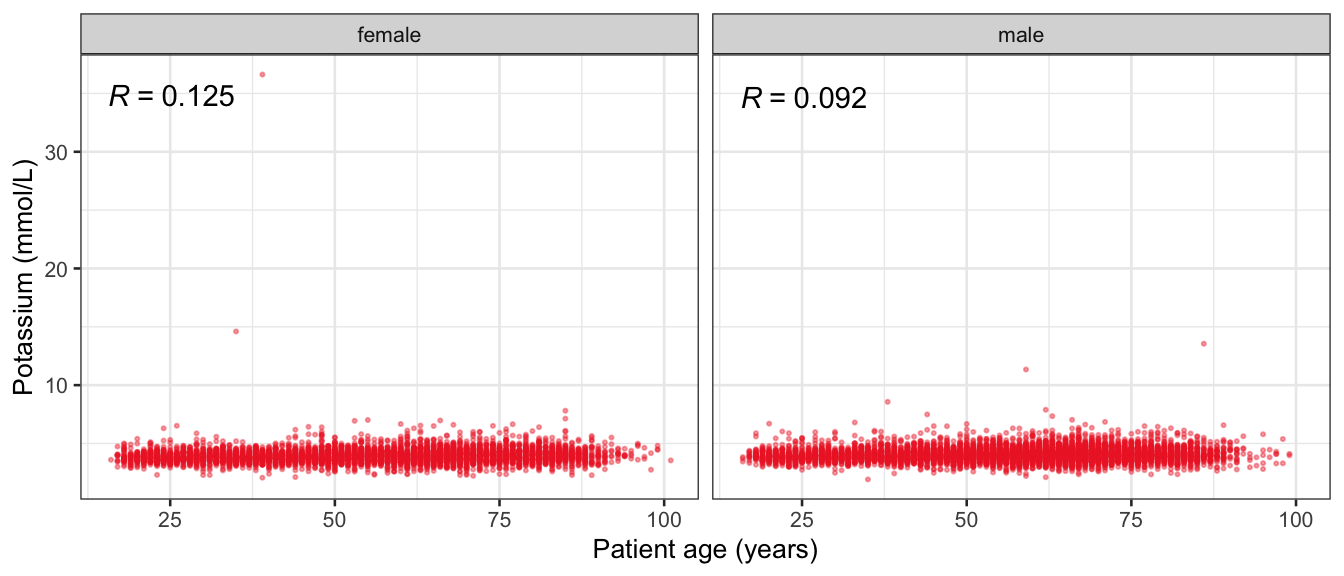
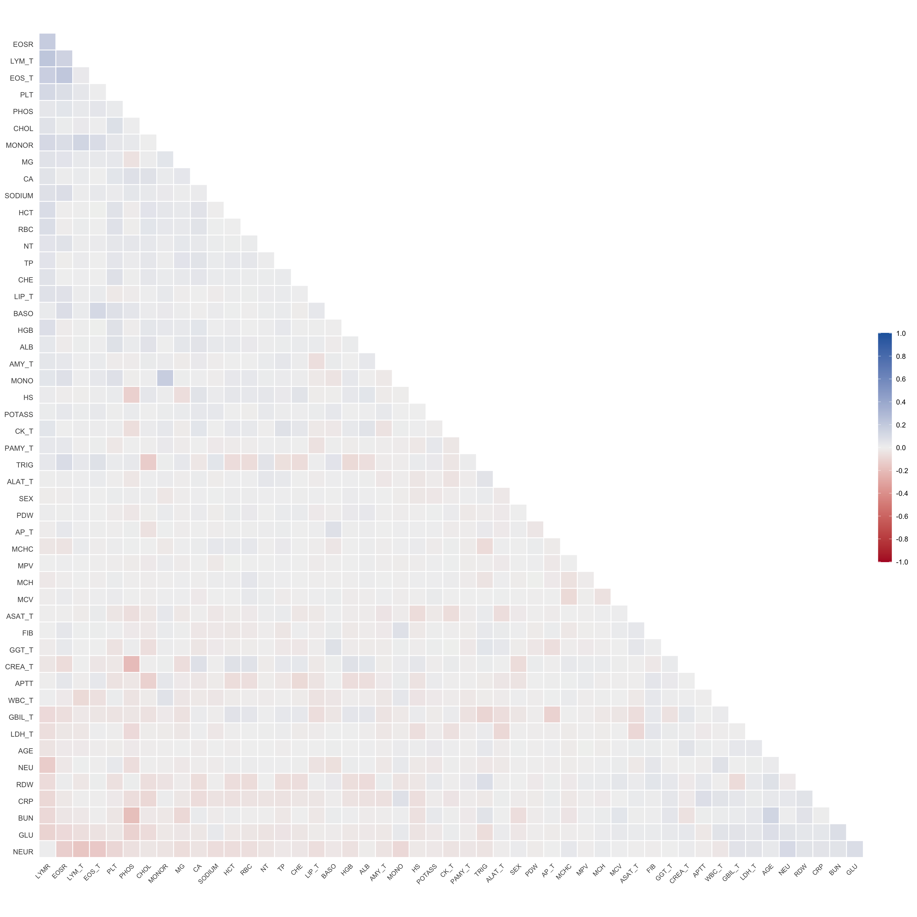
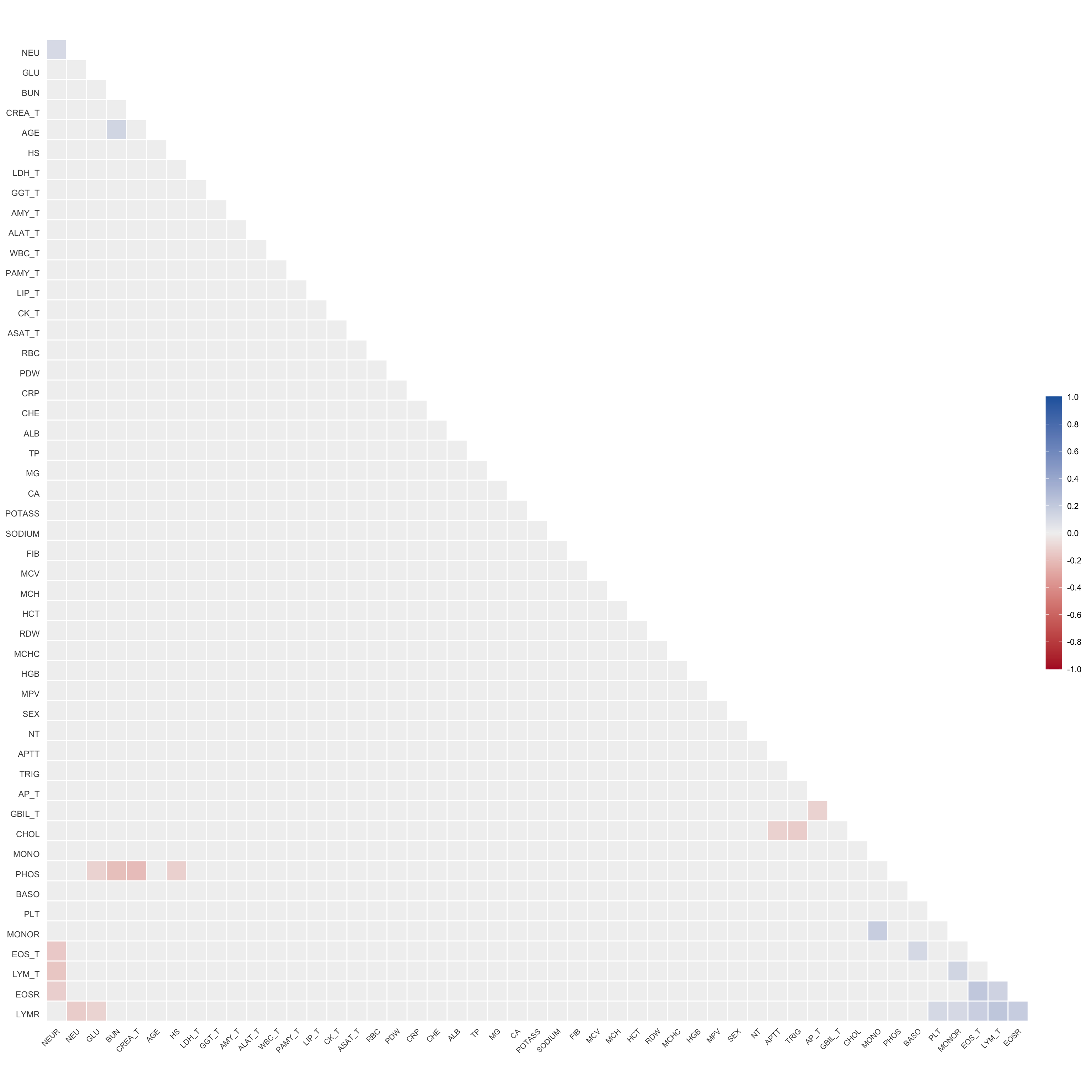
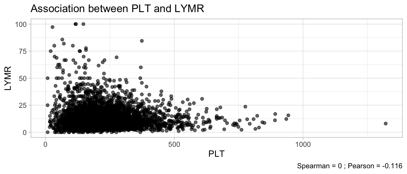
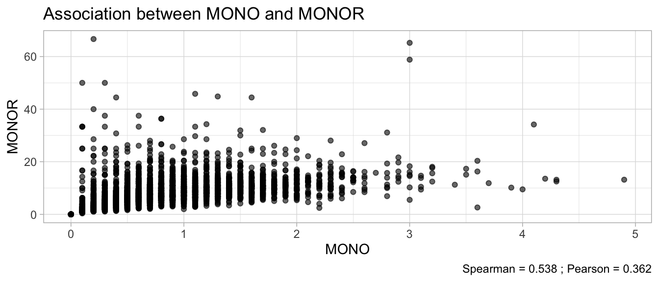
# Multivariate analyses First load the required packages and data. Note that from the univariate analyses the analysis data set for the lab parameters has been updated to include transformed variables. Therefore, we load the second iteration of the data `data/ADLB_02.rds`. ```{r, echo = FALSE, message = FALSE, warning = FALSE } library(tidyr) library(dplyr) library(ggplot2) library(purrr) library(tidyselect) library(corrr) ## tidy correlation library(patchwork) library(ggpubr) library(ggrepel) library(here) library(dendextend) library(gt) library(gtExtras) ## for network plot options(ggrepel.max.overlaps = 100) source(here("R", "fun_compare_dist_plot.R")) source(here("R", "fun_compare_mult_dists.R")) source(here("R", "fun_ida_trans.R")) ## Load the datasets - make sure to load the correct ADLB2 ## TODO: have a make workflow to ensure dependencies run in correct order ADSL <- readRDS(here::here("data","IDA", "ADSL_01.rds")) ADLB <- readRDS(here::here("data","IDA", "ADLB_02.rds")) ``` ## V1: Association with structural variables Attached the required structural variables to the lab data. ```{r mvi01, message=FALSE, warning=FALSE, echo=FALSE, fig.height=3} ## Join with ADSL for structural variables ADSL01 <- ADSL |> select(USUBJID, AGEGR01C, AGE, SEXC, SEX) dat <- ADLB |> left_join(ADSL01, by = "USUBJID") ``` A scatterplot of each predictor with age, with different panels for males and females have been constructed. Associated Spearman correlation coefficients have been computed. The remaining predictors are reported in appendix @sec-V1-appendix. ### Key predictors ```{r mvi03, message=FALSE, warning=FALSE, echo=FALSE, fig.height=3} #| layout-ncol: 2 ## plots for key predictors - remove age to avoid age vs age plot key_predictors <- dat |> filter(!PARAMCD == "AGE") |> filter(KEY_PRED_FL02 == "Y") |> group_by(PARAMCD) |> group_map(~ plot_assoc_by(.x), .keep = TRUE) ## print out. TODO: ask GH which plots to save for (plts in key_predictors) { print(plts) } ``` ### Predictors of medium importance ```{r mvi04, message=FALSE, warning=FALSE, echo=FALSE, fig.height=3} #| layout-ncol: 2 medium_predictors <- dat |> filter(MED_PRED_FL02 == "Y") |> group_by(PARAMCD) |> group_map(~ plot_assoc_by(.x), .keep = TRUE) for (plts in medium_predictors) { print(plts) } ``` ## V2: Correlation coefficients between all predictors Calculate correlation matrix using Spearman correlation coefficient. ```{r mcorrs, message=FALSE, warning=FALSE, echo=FALSE, fig.height=3} ## tidy parameters in to a wide data set dat_wide <- dat |> filter(KEY_PRED_FL02 == "Y" | MED_PRED_FL02 == "Y" | REM_PRED_FL02 == "Y") |> select(USUBJID, PARAMCD, AVAL, SEX) |> pivot_wider(names_from = PARAMCD, values_from = AVAL, values_fill = NA) ## calculate corr matrix using spearman cc corr_spearman <- dat_wide |> select(-USUBJID) |> correlate(use = "pairwise.complete.obs", method = "spearman", diagonal = NA) ``` The Spearman correlation coefficients are depicted in a quadratic heat map: ```{r plotcorr, message=FALSE, warning=FALSE, echo=FALSE, fig.width = 16, fig.height=16} corr_spearman |> rearrange(method = "HC") |> autoplot( # method = "PCA", triangular = "lower", barheight = 20) + theme( axis.text.x = ggplot2::element_text(angle = 45, vjust = 1, hjust = 1, size = 8), axis.text.y = ggplot2::element_text(vjust = 1, hjust = 1, size = 9) ) ``` ```{r} ## If we want to write to file or save # spearman_corr |> # shave(upper = TRUE) |> # fashion() |> # gt::gt() ``` ### VE1: Comparing nonparametric and parametric predictor correlation ```{r corr_setup, message = FALSE, warning = FALSE, echo = FALSE, fig.width = 16, fig.height=16} # differences of pearson and spearman correlations to check for outliers ## cast as a matrix corr_spearman_mat <- corr_spearman |> as_matrix() ## calculate pearson cc corr_pearson <- dat_wide |> select(-USUBJID) |> correlate(use = "pairwise.complete.obs", method = "pearson", diagonal = NA) ## cast as matrix corr_pearson_mat <- corr_pearson |> as_matrix() ## calculate the difference corrd <- corr_spearman_mat - corr_pearson_mat ## cast as tidy data frame TODO: could do this through a join? corr_difference <- corrd |> as_cordf() ``` Plot the matrix of differences between Spearman and Pearson pairwise correlation coefficients. ```{r plotcorr_diff, message=FALSE, warning=FALSE, echo=FALSE, fig.width = 16, fig.height=16} ## plot corr_difference |> rearrange(method = "HC") |> autoplot( # method = "PCA", triangular = "lower", barheight = 20) + theme( axis.text.x = ggplot2::element_text(angle = 45, vjust = 1, hjust = 1, size = 8), axis.text.y = ggplot2::element_text(vjust = 1, hjust = 1, size = 9) ) ``` Plot the matrix of differences between Spearman and Pearson pairwise correlation coefficients but suppress differences less then 0.1 in absolute value. ```{r plotcorr02, message=FALSE, warning=FALSE, echo=FALSE, fig.width = 16, fig.height=16} # sparsified differences of correlation coefficients corr_difference_conditional <- corr_difference |> stretch() |> mutate(r = if_else(abs(r) > 0.1, r, 0)) |> retract() |> as_cordf() ## todo: remove zero entries? corr_difference_conditional |> rearrange(method = "HC") |> autoplot( # method = "PCA", triangular = "lower", barheight = 20) + theme( axis.text.x = ggplot2::element_text(angle = 45, vjust = 1, hjust = 1, size = 8), axis.text.y = ggplot2::element_text(vjust = 1, hjust = 1, size = 9) ) ``` ```{r plotcorr03, message=FALSE, warning=FALSE, echo=FALSE, fig.width = 12, fig.height=12} #corr_difference_conditional |> # shave() |> # rplot(print_cor = TRUE) #corrd_sp <- corrd #corrd_sp[abs(corrd)<0.1] <-0 #ggcorrplot(corrd_sp, tl.cex=5, tl.srt=90) #ggcorrplot(corrd_sp, type = "lower", outline.col = "white") ``` Predictor pairs for which Spearman and Pearson correlation coefficients differ by more than 0.1 correlation units in absolute value will be depicted in scatterplots. First report the table of predictor pairs where the difference (column `r`) is greater than 0.1. ```{r pred_corr, message=FALSE, warning=FALSE, echo=FALSE} ## COMMENT @Mark can we print pearson and spearman correlation coefficients into/over the graphs? combos <- corr_difference_conditional |> shave() |> stretch() |> filter(r > 0.1) combos |> gt::gt() |> gt::fmt_number( columns = c(r), decimals = 2 ) |> gtExtras::gt_theme_538() ``` Then plot the scatter plots. ```{r ve3, message=FALSE, warning=FALSE, echo=FALSE, fig.height=3} #| layout-ncol: 3 ## Data prep combos01 <- combos |> mutate(grp = row_number()) combos_spearman <- corr_spearman |> stretch() |> rename(spearman = r) combos_pearson <- corr_pearson |> stretch() |> rename(pearson = r) combos02 <- combos01 |> left_join(combos_spearman) |> left_join(combos_pearson) ``` ```{r ve3_02, message=FALSE, warning=FALSE, echo=FALSE, fig.height=3} #| layout-ncol: 3 ## Plot the data. source(here("R", "V2-mv-descriptions.R")) combos3 <- combos02 |> group_by(grp) |> group_map(~ plot_scatter_corr(.x), .keep = TRUE) ``` ```{r ve3_03, message=FALSE, warning=FALSE, echo=FALSE, fig.height=3} #| layout-ncol: 3 ## print out. TODO: ask GH which plots to save for (plts in combos3) { print(plts) } ``` ### VE2: Variable clustering A variable clustering analysis has been performed to evaluate which predictors are closely associated. The dendrogram groups predictors by their correlation. ```{r varclust, message=FALSE, warning=FALSE, echo=FALSE, fig.width = 12, fig.height=12} source(here("R", "VE2-varclust.R")) ve2_varclust(corr_spearman) #vc_bact<-Hmisc::varclus(as.matrix(dat)) #plot(vc_bact, cex=0.7, hang=0.01) ``` This can also be displayed as a network plot: ```{r varclust02, message=FALSE, warning=FALSE, echo=FALSE, fig.width = 12, fig.height=8} #options(ggrepel.max.overlaps = 100) corr_spearman |> network_plot() ``` ```{r varclust03, message=FALSE, warning=FALSE, echo=FALSE, fig.width = 12, fig.height=6} # plot network with min cor of 0.3. # corr_spearman |> network_plot(min_cor = 0.3) ``` In the following scatterplots we show predictor pairs with Spearman correlation coefficients greater than 0.8: ```{r varclust04, message=FALSE, warning=FALSE, echo=FALSE, fig.width = 12, fig.height=6} combos_spearman_02 <- corr_spearman |> shave() |> stretch() |> rename(spearman = r) |> filter(abs(spearman) > 0.8) |> mutate(grp = row_number()) ``` ```{r varclust05, message=FALSE, warning=FALSE, echo=FALSE, fig.height=3} #| layout-ncol: 2 source(here("R", "V2-mv-descriptions.R")) combos_spearman_03 <- combos_spearman_02 |> group_by(grp) |> group_map(~ plot_scatter_corr(.x, pearson_flag = FALSE), .keep = TRUE) ## print out. TODO: ask GH which plots to save for (plts in combos_spearman_03 ) { print(plts) } ``` ### VE3: Redundancy Variance inflation factors (VIF) will be computed between the candidate predictors. This will be done for the three possible candidate models, and using all complete cases in the respective candidate predictor sets. Since $VIF = (1-R^2)^{-1}$, we also report the multiple R-squared values. Redundancy was further explored by computing parametric additive models for each predictor in the key predictor model and the extended predictor model. VIFs and multiple $R^2$ are reported from those models, again for the three predictor sets. Note, the all predictor model is reported in appendix @sec-VE3-appendix. #### VIF for key predictor model ```{r vif, message=FALSE, warning=FALSE, echo=FALSE, fig.height=3} dat_wide <- dat |> filter(KEY_PRED_FL02 == "Y") |> select(USUBJID, PARAMCD, AVAL, SEX) |> pivot_wider(names_from = PARAMCD, values_from = AVAL, values_fill = NA) dat_vif <- dat_wide |> select(-USUBJID) formula <- as.formula(paste(c("~",paste(names(dat_vif), collapse="+")), collapse="")) #formula red <- Hmisc::redun(formula, data = dat_vif, nk=0, pr=FALSE) vif <- 1/(1-red$rsq1) #cat("\nAvailable samvple size:\n", red$n, " (", #round(100*red$n/nrow(dat),2), "%)\n") vif_df <- as_tibble(vif, rownames = "PARAMCD") |> rename(vif = value) red_df <- as_tibble(red$rsq1, rownames = "PARAMCD") |> rename(r2 = value) tab_df <- vif_df |> left_join(red_df, by = "PARAMCD") ``` The available sample size is `r red$n` (`r round(100*red$n/nrow(dat),2)` %). ```{r vif02, message=FALSE, warning=FALSE, echo=FALSE, fig.height=3} #vif_df |> gt::gt(caption = "Variance inflation factors") #red_df |> gt::gt(caption = "Multiple R-squared") tab_df |> gt() |> gt::cols_label( PARAMCD = "Parameter code", r2 = "Multiple R-squared", vif = "Variance inflation factor" ) |> fmt_number( columns = c(r2), decimals = 2 ) |> fmt_number( columns = c(vif), decimals = 1 ) |> gt_theme_538() ``` #### VIF for model with key predictors and predictors of medium importance ```{r vif03, message=FALSE, warning=FALSE, echo=FALSE, fig.height=3} dat_wide <- dat |> filter(KEY_PRED_FL02 == "Y" | MED_PRED_FL02 == "Y") |> select(USUBJID, PARAMCD, AVAL, SEX) |> pivot_wider(names_from = PARAMCD, values_from = AVAL, values_fill = NA) dat_vif <- dat_wide |> select(-USUBJID) formula <- as.formula(paste(c("~",paste(names(dat_vif), collapse="+")), collapse="")) #formula red <- Hmisc::redun(formula, data = dat_vif, nk=0, pr=FALSE) vif <- 1/(1-red$rsq1) #cat("\nAvailable samvple size:\n", red$n, " (", #round(100*red$n/nrow(dat),2), "%)\n") vif_df <- as_tibble(vif, rownames = "PARAMCD") |> rename(vif = value) red_df <- as_tibble(red$rsq1, rownames = "PARAMCD") |> rename(r2 = value) tab_df <- vif_df |> left_join(red_df, by = "PARAMCD") ``` The available sample size is `r red$n` (`r round(100*red$n/nrow(dat),2)` %). ```{r vif04, message=FALSE, warning=FALSE, echo=FALSE, fig.height=3} #vif_df |> gt::gt(caption = "Variance inflation factors") #red_df |> gt::gt(caption = "Multiple R-squared") tab_df |> gt() |> gt::cols_label( PARAMCD = "Parameter code", r2 = "Multiple R-squared", vif = "Variance inflation factor" ) |> fmt_number( columns = c(r2), decimals = 2 ) |> fmt_number( columns = c(vif), decimals = 1 ) |> gt_theme_538() ``` #### VIF for all predictor model See appendix @sec-VE3-appendix. #### Redundancy by parametric additive model: key predictor model ```{r key_vif, message=FALSE, warning=FALSE, echo=FALSE, fig.height=3} dat_wide <- dat |> filter(KEY_PRED_FL02 == "Y") |> select(USUBJID, PARAMCD, AVAL, SEX) |> pivot_wider(names_from = PARAMCD, values_from = AVAL, values_fill = NA) dat_vif <- dat_wide |> select(-USUBJID) formula <- as.formula(paste(c("~",paste(names(dat_vif), collapse="+")), collapse="")) red <- Hmisc::redun(formula, data = dat_vif, pr=FALSE) vif <- 1/(1-red$rsq1) #cat("\nAvailable samvple size:\n", red$n, " (", #round(100*red$n/nrow(dat),2), "%)\n") vif_df <- as_tibble(vif, rownames = "PARAMCD") |> rename(vif = value) red_df <- as_tibble(red$rsq1, rownames = "PARAMCD") |> rename(r2 = value) tab_df <- vif_df |> left_join(red_df, by = "PARAMCD") ``` The available sample size is `r red$n` (`r round(100*red$n/nrow(dat),2)` %). ```{r key_vif02, message=FALSE, warning=FALSE, echo=FALSE, fig.height=3} #vif_df |> gt::gt(caption = "Variance inflation factors") #red_df |> gt::gt(caption = "Multiple R-squared") tab_df |> gt() |> gt::cols_label( PARAMCD = "Parameter code", r2 = "Multiple R-squared", vif = "Variance inflation factor" ) |> fmt_number( columns = c(r2), decimals = 2 ) |> fmt_number( columns = c(vif), decimals = 1 ) |> gt_theme_538() ``` #### Redundancy by parametric additive model: key predictors and predictors of medium importance ```{r key_vif03, message=FALSE, warning=FALSE, echo=FALSE, fig.height=3} dat_wide <- dat |> filter(KEY_PRED_FL02 == "Y" | MED_PRED_FL02 == "Y") |> select(USUBJID, PARAMCD, AVAL, SEX) |> pivot_wider(names_from = PARAMCD, values_from = AVAL, values_fill = NA) dat_vif <- dat_wide |> select(-USUBJID) formula <- as.formula(paste(c("~",paste(names(dat_vif), collapse="+")), collapse="")) #formula red <- Hmisc::redun(formula, data = dat_vif, pr=FALSE) vif <- 1/(1-red$rsq1) #cat("\nAvailable samvple size:\n", red$n, " (", #round(100*red$n/nrow(dat),2), "%)\n") vif_df <- as_tibble(vif, rownames = "PARAMCD") |> rename(vif = value) red_df <- as_tibble(red$rsq1, rownames = "PARAMCD") |> rename(r2 = value) tab_df <- vif_df |> left_join(red_df, by = "PARAMCD") ``` The available sample size is `r red$n` (`r round(100*red$n/nrow(dat),2)` %). ```{r key_vif04, message=FALSE, warning=FALSE, echo=FALSE, fig.height=3} #vif_df |> gt::gt(caption = "Variance inflation factors") #red_df |> gt::gt(caption = "Multiple R-squared") tab_df |> gt() |> gt::cols_label( PARAMCD = "Parameter code", r2 = "Multiple R-squared", vif = "Variance inflation factor" ) |> fmt_number( columns = c(r2), decimals = 2 ) |> fmt_number( columns = c(vif), decimals = 1 ) |> gt_theme_538() ```